AI how-to notes · 2026-09-18 · last run 2026-09-18 · 한국어 원문
Excel $ absolute references — how a quote's tax column became 0, #VALUE! and 3,264,000,000
One line summary
Write the VAT rate into the single cell D1, compute tax with =D4*D1, copy it down, and from the second row onward D2, D3 and D4 land in the rate's place. Across five rows of a dummy quote the tax came out as 2400 → 0 → #VALUE! → 3,264,000,000 → 2,625,000,000, and the total was #VALUE!. The column fixed to =D4*$D$1 totalled 28,400.
Symptoms
- The first row is right, and from the second row the numbers go to 0 or blow up
- You copied the formula and got
#VALUE! - The tax total comes out as
#VALUE! - Looking at the formula bar, a cell you never picked is in there
Test environment
| Item | Value |
|---|---|
| OS | Windows 11 Home (10.0.26200) |
| Excel | 16.0 (build 20326.0) |
| How we drove it | Excel COM (Excel.Application, Visible=false). We wrote formula strings into cells, and copied with Range.Copy + Range.PasteSpecial(xlPasteAll). This is not a test of pressing F4 on a keyboard |
| Test file | Our own dummy X1_42_견적서.xlsx |
| Logs | 원자료\excel-absolute-reference\01_absolute_실행로그.txt, 02_png_렌더로그.txt (the scripts X1_42_absolute.py and X1_42_png.py are in the same folder) |
The dummy quote
The VAT rate went into the single cell D1 as 10%, with five line items below it. The net amount (column D) came from =B4*C4 in D4, copied into D5:D8. The pasted cells held =B5*C5 through =B8*C8 and every value matched that row's quantity × unit price, because those are references that are supposed to travel down with the row.
We calculated the tax two ways. Column E got =D4*D1 copied down; column F got =D4*$D$1 copied the same way.
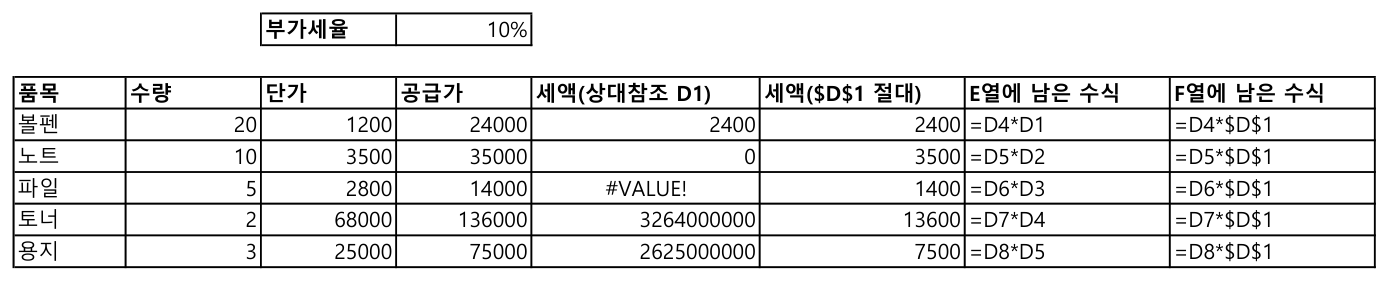
| Item | Qty | Unit price | Net | Tax E (=D4*D1 copied) | Formula left in E | What landed in the rate's place | Tax F ($D$1) |
|---|---|---|---|---|---|---|---|
| 볼펜 | 20 | 1200 | 24000 | 2400 | =D4*D1 | D1 = 10% | 2400 |
| 노트 | 10 | 3500 | 35000 | 0 | =D5*D2 | D2 = (empty) | 3500 |
| 파일 | 5 | 2800 | 14000 | #VALUE! | =D6*D3 | D3 = the text 「공급가」 | 1400 |
| 토너 | 2 | 68000 | 136000 | 3264000000 | =D7*D4 | D4 = 24000 | 13600 |
| 용지 | 3 | 25000 | 75000 | 2625000000 | =D8*D5 | D5 = 35000 | 7500 |
(The items are ballpoint pen, notebook, folder, toner and paper; 「공급가」 is the "net amount" column header.)
| Total | Formula | Value |
|---|---|---|
| Net | =SUM(D4:D8) | 284,000 |
| Tax (relative, column E) | =SUM(E4:E8) | #VALUE! |
Tax ($D$1, column F) | =SUM(F4:F8) | 28,400 |
Only the first row was right. The second row's rate slot took the empty D2, so it multiplied by 0; the third took the header text 「공급가」 and became #VALUE!. The fourth and fifth took the net amount from the row above into the rate slot and ran into the billions.
The row worth staring at is the second. A 0 carries no error marker. We built a separate case to see what happens when the displaced cell holds another rate rather than a blank — a table with the VAT rate 0.1 in D1 and last month's discount rate 0.05 still sitting directly below it in D2.
| Item | Net | Tax (relative) | Formula in that cell | Tax ($D$1) |
|---|---|---|---|---|
| 볼펜 | 24000 | 2400 | =D4*D1 | 2400 |
| 노트 | 35000 | 1750 | =D5*D2 | 3500 |
The second row is 35,000 × 0.05 = 1,750. No error marker, and the amount is plausible. It is half the correct 3,500, and without a cross-check it goes out as-is. #VALUE! and the 3.2 billion are, if anything, the merciful ones.
Why it happens
An address without $ is remembered as "so many cells away". Copying rewrites the address to preserve that distance. =D4*D1 in E4 means "one cell to my left × one cell to the left of three cells above me", and moving that formula to E5 shifts each part down one row, giving =D5*D2.
The net-amount formula =B4*C4 copied without trouble because the cells it points at are supposed to travel down with the row. The problem is a value like a tax rate that must be read from one cell no matter where you look at it from. Put a $ in front of the column letter or the row number and that part stops moving when copied.
Comparing $D$1, $D1 and D$1 by their results
We put different values in the nine cells C1:E3 and used D1 as the reference cell. C1=100, D1=10, E1=1000 / C2=200, D2=20, E2=2000 / C3=300, D3=30, E3=3000. Making every value different means the number alone tells you which cell the copied formula grabbed.
We put each of four formulas in one cell and copied it into a 3-wide × 3-tall range including that cell.
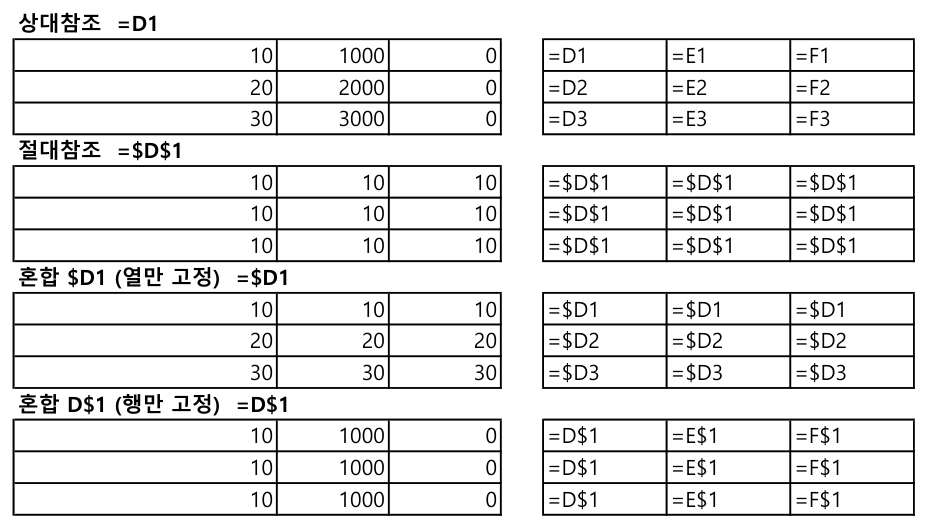
`=D1`, relative — it moves both horizontally and vertically. The rightmost column picked up F1, F2 and F3, which had no values, and came out 0.
| Col 1 | Col 2 | Col 3 | |
|---|---|---|---|
| Row 1 | 10 (=D1) | 1000 (=E1) | 0 (=F1) |
| Row 2 | 20 (=D2) | 2000 (=E2) | 0 (=F2) |
| Row 3 | 30 (=D3) | 3000 (=E3) | 0 (=F3) |
`=$D$1`, absolute — all nine cells are 10. The formula is =$D$1 in all nine as well.
| Col 1 | Col 2 | Col 3 | |
|---|---|---|---|
| Row 1 | 10 | 10 | 10 |
| Row 2 | 10 | 10 | 10 |
| Row 3 | 10 | 10 | 10 |
`=$D1`, mixed, column locked — copied sideways it stays on column D; copied down it follows the rows.
| Col 1 | Col 2 | Col 3 | |
|---|---|---|---|
| Row 1 | 10 (=$D1) | 10 (=$D1) | 10 (=$D1) |
| Row 2 | 20 (=$D2) | 20 (=$D2) | 20 (=$D2) |
| Row 3 | 30 (=$D3) | 30 (=$D3) | 30 (=$D3) |
`=D$1`, mixed, row locked — copied down it stays on row 1; copied sideways it moves along.
| Col 1 | Col 2 | Col 3 | |
|---|---|---|---|
| Row 1 | 10 (=D$1) | 1000 (=E$1) | 0 (=F$1) |
| Row 2 | 10 (=D$1) | 1000 (=E$1) | 0 (=F$1) |
| Row 3 | 10 (=D$1) | 1000 (=E$1) | 0 (=F$1) |
$ pins only what comes immediately after it. $D pins the column; the $1 in D$1 pins the row. In a quote sheet, where you only ever copy up and down, D$1 gives the same values as $D$1 — the row is pinned, so going down still reads row 1. But copy that column one cell sideways later and it becomes E$1 and diverges. For a value that must always be read from one cell, pinning both with $D$1 saves trouble down the line.
Where a mixed reference beats an absolute one
In a table you fill in two directions at once, $D$1 is the wrong answer. We built a table with quantity down the left (column A), unit price across the top (row 1), and the body to be filled in. The top-left cell got =$A2*B$1, copied across 3 × 3.

| Qty↓ / Price→ | 1000 | 2000 | 5000 |
|---|---|---|---|
| 1 | 1000 (=$A2*B$1) | 2000 (=$A2*C$1) | 5000 (=$A2*D$1) |
| 5 | 5000 (=$A3*B$1) | 10000 (=$A3*C$1) | 25000 (=$A3*D$1) |
| 10 | 10000 (=$A4*B$1) | 20000 (=$A4*C$1) | 50000 (=$A4*D$1) |
All nine cells came out as that row's quantity times that column's price. $A2 pins the column because the quantity always lives in column A and leaves the row free; B$1 pins the row because the price always lives in row 1 and leaves the column free.
Put =A2*B1 in the same cell and copy it identically and you get this.
| Col 2 | Col 3 | Col 4 | |
|---|---|---|---|
| Row 1 | 1,000 (=A2*B1) | 2,000,000 (=B2*C1) | 10,000,000,000 (=C2*D1) |
| Row 2 | 5,000 (=A3*B2) | 10,000,000,000 (=B3*C2) | 1E+20 (=C3*D2) |
| Row 3 | 50,000 (=A4*B3) | 5E+14 (=B4*C3) | 5E+34 (=C4*D3) |
Only two cells hold the right value, 1,000 and 5,000. Each cell becomes "the cell to the left × the cell above", so values explode toward the bottom right and Excel shows them in scientific notation such as 1E+20. (Corrected 2026-09-28 — the table as first published did not match the multiplication.) =A3*B2 came out as 5000 by coincidence, because the value already sitting in B2 (1×1000) happened to be 1000. In the other seven cells at least one of the two references has moved off the header and into a calculated result inside the table.
Naming the cell instead of using $
You can also give the reference cell a name. In this test we registered the name 「부가세율」 (VAT rate) over COM, pointing at 견적서!$D$1 — an absolute reference.
=D4*부가세율Here is that formula put in H4 and copied into H5:H8.
| Cell | Formula | Value |
|---|---|---|
| H4 | =D4*부가세율 | 2400 |
| H5 | =D5*부가세율 | 3500 |
| H6 | =D6*부가세율 | 1400 |
| H7 | =D7*부가세율 | 13600 |
| H8 | =D8*부가세율 | 7500 |
The same values as column F ($D$1). The advantage is that the formula alone tells you what is being multiplied.
We also checked what happens when the reference cell moves. On a second sheet we put 0.1 in B1, registered the name 「세율2」 (rate 2) as 이름이동!$B$1, and got 100 from =1000*세율2. Then we cut B1 and pasted it into B10.
| Where the name points | =1000*세율2 | |
|---|---|---|
| Before the move | =이름이동!$B$1 | 100 |
| After moving B1 to B10 | =이름이동!$B$10 | 100 |
The name followed the cell, so the value held without touching the formula. If you are building a quote sheet you intend to reuse as a template, this is the one we would recommend.
How to check after copying
Start by clicking three cells. Click the first row, one row in the middle and the last row, and read the formula bar. Check that the reference cell's address and its $ marks are identical in all three. If even one differs, the reference slid somewhere in between. Three matching cells are no guarantee the whole column is right, so with many rows, lay them all out with FORMULATEXT below.
To see it all on one screen, put FORMULATEXT in the cell next door. Every cell labelled "formula" in this note's screenshots came from this function.
=FORMULATEXT(E4)Cross-check with numbers too. In this quote, check whether 10% of the net total of 284,000 — that is, 28,400 — matches the tax total.
=SUM(D4:D8)*D1   → 28400
=SUM(F4:F8)      → 28400
If the two differ, something has slipped. A row with a slid reference is the common cause, and the total's range may also be wrong.
What failed
- While printing the 3×3 copy results we called
cell.Address(False, False)and the script died partway withTypeError: 'str' object is not callable. On this pywin32 binding,Addresscomes through as a value, not a function. The log file is written in one go at the end of the script, so that aborted run left no file; we read the exception on screen, built the addresses ourselves and re-ran. The fixed code is inX1_42_absolute.pyas it stands. - We could not test cycling through
$placements with the F4 key. Every result in this note came from writing formula strings directly into cells. We did not check the order in which F4 applies$, so we did not write about it. - A fact-check pass with GPT on the draft (result at
대조결과\excel-absolute-reference_1차.md) flagged "copying only up and down makes$D1equal to$D$1" as contradicting the log. The log showed$D1turning into$D2and$D3as it was copied down, giving 10, 20, 30. The one that matches$D$1under vertical copying isD$1. We corrected the text. - The same pass flagged "only the first cell of the relative-reference table is right" as contradicting the log too. Recounting, two cells matched the expected value, B2 and B3, and the second was a coincidence. We corrected the number in the text.
- Two sentences — "a named cell follows when you move the reference cell" and "if a small number sits in the displaced slot you get a plausible amount with no error" — were flagged as guesswork we had not run. We ran both for real, recorded them as items (타) and (카) in the execution log, and put them into the tables above.
What we did not test
- We ran on one build only, Excel 16.0 build 20326.0. We did not check 2016 or 2019, Excel for the web, or Google Sheets.
- What happens to references when you move a formula cell by cutting it (Ctrl+X) was not tested. Cutting was only used on the named reference cell.
- Dragging the fill handle with the mouse was not reproduced over COM. These results are based on
Range.Copy+PasteSpecial. - Structured references used inside an Excel table (things like
[@수량]) were not tried. - The behaviour of copying a reference that points at another sheet or another file was not tested.
- How things appear when the workbook is switched to R1C1 reference style was not checked.
- Registering a name through the name box or the formula tab on screen was not clicked through on this build. Every name here was registered over COM.