AI how-to notes · 2026-09-18 · last run 2026-09-18 · 한국어 원문
Comparing two lists in Excel — COUNTIF for common and one-sided entries, and the cases where it lies
One line summary
To reconcile two lists you need =COUNTIF(other list, my value) on both sheets. Put it on one side only and anyone who exists solely on the other list never appears on screen at all. Running it against dummy lists of 8 employee numbers each, the correct answer is 6 common, 2 only in A and 2 only in B, while the formulas reported 5 common, 3 only in A and 3 only in B — and the one mismatch came down to a single trailing space after an employee number.
Who this is for
- Anyone matching a personnel roster against a training completion list to pull out who has not taken it yet
- Anyone handed two vendor lists who has to pick out the overlap
- Anyone who ran VLOOKUP, got a pile of
#N/A, and does not know how far to trust it
Test environment
| Item | Value |
|---|---|
| OS | Windows 11 Home (10.0.26200) |
| Excel | 16.0 (build 20326) |
| Method | Excel COM (Excel.Application, Visible=false) |
| Test file | A dummy we built ourselves, E2_25_명단비교.xlsx — sheets 명단A and 명단B (list A, list B), 8 rows each |
| Logs | 원자료\excel-compare-two-lists\01_비교_실행로그.txt, 02_trim_다시세기.txt, 03_보탬시험.txt |
We wrote down the answer first
Before running any formula we nailed the by-eye answer into the log, so that we would have something to hold the formula results against later.
- 6 in common — A1001, A1002, A1003, A1005, A1006 (lowercase a1006 in A), 1007
- 2 only in 명단A — A1004, A1008
- 2 only in 명단B — A1009, A1010
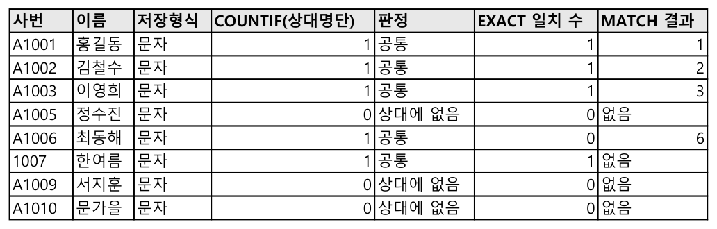
We planted three flaws in 명단B that show up constantly in real work: a single trailing space after A1005 (A1005 ), the a1006 that is lowercase in 명단A written as uppercase A1006, and the employee number 1007 stored as a number in 명단A written as the text "1007".
Put the same formula on both sides
This is what went into column D of the 명단A sheet.
=COUNTIF(명단B!$A$2:$A$9,A2)
=IF(D2=0,"상대에 없음","공통")
The 명단B sheet gets the same thing with the direction reversed. (The two labels read "not on the other side" and "common".)
=COUNTIF(명단A!$A$2:$A$9,A2)To see what exactly goes wrong we added two more. EXACT looks at case as well, and MATCH looks at whether the cell stores a number or text.
=SUMPRODUCT(--EXACT(A2,명단B!$A$2:$A$9))
=IFERROR(MATCH(A2,명단B!$A$2:$A$9,0),"없음")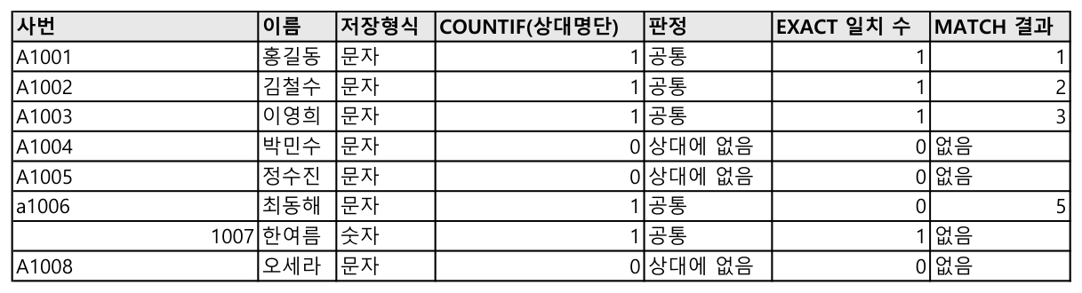
The three give different answers
| Employee no. (명단A) | Stored as | COUNTIF | EXACT matches | MATCH | How it looks on the other list |
|---|---|---|---|---|---|
| A1001 | text | 1 | 1 | 1 | identical |
| A1002 | text | 1 | 1 | 2 | identical |
| A1003 | text | 1 | 1 | 3 | identical |
| A1004 | text | 0 | 0 | 없음 | not on the other list |
| A1005 | text | 0 | 0 | 없음 | A1005 — one trailing space |
| a1006 | text | 1 | 0 | 5 | A1006 — uppercase |
| 1007 | number | 1 | 1 | 없음 | "1007" — stored as text |
| A1008 | text | 0 | 0 | 없음 | not on the other list |
Look at where the three part ways. (없음 is the "not found" label our IFERROR supplies.)
One trailing space (A1005). To a human it is the same employee number, and all three — COUNTIF, EXACT and MATCH — failed to find it. The characters on screen are the same, but the cells hold 5 characters and 6. From the 명단A side it reads "not in B" and from the 명단B side "not in A", so the same person lands on both missing-person lists at once.
Case (a1006). COUNTIF counted 1 and called it common; EXACT returned 0. COUNTIF does not distinguish upper from lower case. For employee numbers that behavior is convenient, but for code values where case carries meaning (product codes AB-1 versus ab-1) you need EXACT.
Number versus text (1007). COUNTIF says 1, MATCH says not found. COUNTIF treated the number 1007 and the text "1007" as the same value; MATCH's exact match (third argument 0) did not. We put VLOOKUP in the same spot too.
=IFERROR(VLOOKUP(A2,명단B!$A$2:$B$9,2,FALSE),"#N/A")| Employee no. | COUNTIF | MATCH | VLOOKUP |
|---|---|---|---|
| A1001 | 1 | 1 | 홍길동 |
| A1002 | 1 | 2 | 김철수 |
| A1003 | 1 | 3 | 이영희 |
| A1004 | 0 | 없음 | #N/A |
| A1005 | 0 | 없음 | #N/A |
| a1006 | 1 | 5 | 최동해 |
| 1007 | 1 | 없음 | #N/A |
| A1008 | 0 | 없음 | #N/A |
Look at the 1007 line. COUNTIF counts it as present while VLOOKUP returns #N/A. This is exactly where "the person is on the list, so why can't it fetch the name?" comes from. The case-only difference, a1006, was found by all three of COUNTIF, MATCH and VLOOKUP.
What the formulas counted vs what a human counted
| What was counted | Formula result | Correct | Formula used |
|---|---|---|---|
| Common, from A | 5 | 6 | =COUNTIF(D2:D9,">0") |
| Only in A | 3 | 2 | =COUNTIF(D2:D9,0) |
| Common, from B | 5 | 6 | =COUNTIF(명단B!D2:D9,">0") |
| Only in B | 3 | 2 | =COUNTIF(명단B!D2:D9,0) |
| EXACT matches in A | 4 | — | =COUNTIF(F2:F9,">0") |
| MATCH hits in A | 4 | — | =COUNT(G2:G9) |
| Rows in A | 8 | 8 | =COUNTA(A2:A9) |
| Rows in B | 8 | 8 | =COUNTA(명단B!A2:A9) |
Each side is off by one, and that one is A1005. Seen from either direction it reads "not on the other side", so it gets caught twice.
Counting again with the space stripped
We added one cleanup column on each side, stripped the leading and trailing spaces with TRIM, and compared those columns against each other.
I2: =TRIM(A2)
J2: =COUNTIF(명단B!$I$2:$I$9,I2)
| What was counted | Before cleanup | After cleanup | Correct |
|---|---|---|---|
| Common, from A | 5 | 6 | 6 |
| Only in A | 3 | 2 | 2 |
One TRIM brought it in line with the correct answer. The case difference between a1006 and A1006, and the number-versus-text split on 1007, were already being counted as matches by the pre-cleanup COUNTIF, so there was nothing to fix there. Better to build this cleanup column the moment a list arrives.
Counting the characters in the cell shows a stray space immediately.
=LEN(A2)In the test file, A1005 in 명단A was 5 and A1005 in 명단B was 6. That one-character gap is what threw off COUNTIF, EXACT, MATCH and VLOOKUP alike. When the visible characters match but the lengths differ, start your suspicion with that cell.
What failed
- Building the cleanup column the first time, we set the cell format to 「텍스트」 (Text) first and then entered
=TRIM(A2). The formula did not calculate, stayed as literal text, and COUNTIF returned 0 for all 8 rows. Clearing the format and re-entering it put things right. Do not pre-apply text format to cells that are going to hold formulas. - Trying to reset the format,
NumberFormat = "General"over COM was refused with 「Range 클래스 중 NumberFormat 속성을 설정할 수 없습니다」 — "unable to set the NumberFormat property of the Range class". On Korean Excel the same format is namedG/표준. We solved it by clearing the format withClearFormats()instead, after which readingNumberFormatLocalgaveG/표준. - We did not try the 홈 > 조건부 서식 > 중복 값 (Home > Conditional Formatting > Duplicate Values) route that colors both lists on one screen.
- We failed to record the formulas as entered on the 명단B sheet in the first log, so we read them back later and appended them to
03_보탬시험.txt.
What we did not test
- We did not try a space in the middle of an employee number (
A10 05). TRIM collapses interior runs of spaces to one; it does not remove them. - Other invisible characters (line breaks, full-width spaces, Unicode 160) were not part of the test. The cases where
CLEANorSUBSTITUTEare needed live here. - We did not measure how much COUNTIF in both directions slows down on lists of several thousand rows. We only checked with 8 rows.
- We did not compare the results of doing the same job with newer functions such as XLOOKUP or FILTER.
- We did not check how Power Query's merge (join) handles a single trailing space.